graph LR
    IM["Ice Mass"]       -->|"+"| SA["Surface Albedo"]
    SA                   -->|"−"| SR["Solar Absorption"]
    SR                   -->|"+"| ST["Surface Temperature"]
    ST                   -->|"+"| MR["Ice Melt Rate"]
    MR                   -->|"− [R]"| IM

    style IM fill:#f5f5f5,stroke:#111111,stroke-width:2px
    style SA fill:#f5f5f5,stroke:#111111,stroke-width:2px
    style SR fill:#f5f5f5,stroke:#111111,stroke-width:2px
    style ST fill:#f5f5f5,stroke:#111111,stroke-width:2px
    style MR fill:#fff3f3,stroke:#d52a2a,stroke-width:2px
3 Feedback Structures
Reinforcing loops, balancing loops, and the behaviour they generate
3.1 The puzzle
You receive a bonus. You invest it. The investment earns returns. You reinvest the returns. The returns earn returns on returns. Forty years later, the original bonus is a small fraction of the total.
You are treated for a bacterial infection. A subset of bacteria survive the antibiotic. They reproduce. Their resistant offspring survive the next antibiotic treatment. The subset grows. A decade later, the antibiotic no longer works.
A city attracts a cluster of technology firms. Workers follow. More firms locate there to access the workers. More workers follow the firms. Infrastructure investment makes the city more attractive. Two decades later, housing is unaffordable, but firms still come because the workers are there.
Three different domains. The same underlying structure. Each is a reinforcing loop (Meadows 2008) — a feedback structure where a change in a stock leads to a flow that amplifies the change. They are not just metaphorically similar. They are governed by the same mathematical relationship, generating the same characteristic behaviour.
3.2 Two types of feedback
In Chapter 1 we saw that a system’s behaviour over time is produced by its stock-flow structure. But that structure has another layer: feedback loops — connections that close the circle between a stock’s current state and the flows that change it.
There are exactly two types of feedback loop:
Reinforcing (positive) feedback: A change in the stock produces flows that move the stock further in the same direction. Growth feeds growth. Decline feeds decline. Reinforcing loops generate exponential dynamics — accelerating growth or accelerating collapse.
Balancing (negative) feedback: A change in the stock produces flows that oppose the change. A departure from a goal produces a corrective flow. Balancing loops generate goal-seeking behaviour — the system tends toward an equilibrium or target.
The language here is confusing. “Positive feedback” in common usage means something desirable. In systems thinking it means something that amplifies. “Negative feedback” means something that opposes — in engineering, this is often exactly what you want (a thermostat is negative feedback; it keeps temperature stable). Neither is inherently good or bad. Ask instead: good or bad for what purpose?
3.3 Reinforcing loops
A reinforcing loop exists when a change in the stock reinforces itself through the flow structure.
The simplest version: a bank account with compound interest.
\frac{dS}{dt} = r \cdot S
where S is the account balance and r is the interest rate. The inflow (interest earned) is proportional to the stock itself. The more you have, the more you earn.
This generates exponential growth:
S(t) = S_0 \cdot e^{rt}
The same equation, with a negative r, generates exponential decay (radioactive decay, drug elimination, equipment depreciation).
3.3.1 The ice-albedo feedback (Earth systems)
Ice is white. It reflects about 80–90% of incoming solar radiation. Open ocean and bare rock are dark — they absorb 80–90%.
When ice melts, it exposes darker surfaces. Those surfaces absorb more heat. That heat melts more ice. The loop:
Figure 2.1. Ice-albedo reinforcing loop. Two negative causal links and three positive links produce a reinforcing (R) loop: any reduction in ice mass ultimately produces further reduction. Notation: a + label means cause and effect move in the same direction. A − label means they move in opposite directions. A loop is reinforcing (R) when it contains an even number of − signs; balancing (B) when it contains an odd number.
This is a reinforcing loop. A small warming perturbation, amplified through this loop, produces greater warming than the original forcing alone would suggest.
It is not unlimited — other feedbacks intervene, and the ice-albedo feedback eventually runs out of ice to melt. But the Arctic, which has lost roughly 40% of its September sea ice extent since satellite records began (Stroeve et al. 2012), is partly running this loop in real time.
3.3.2 Agglomeration in cities (Human systems)
Why are certain cities much larger than others? Why does a given industry cluster in a few places rather than spreading evenly? The answer involves reinforcing feedback (Krugman 1991).
A city with skilled workers is attractive to firms that need skilled workers. Those firms offer jobs, attracting more skilled workers. More workers make the city more attractive to more firms. The city develops specialised suppliers, contractors, and training institutions. These lower the cost of doing business, making the city more attractive still.
graph LR
    SW["Skilled Workers"]    -->|"+"| FC["Firm Concentration"]
    FC                       -->|"+"| JA["Job Availability"]
    JA                       -->|"+ [R]"| SW

    style SW fill:#f5f5f5,stroke:#111111,stroke-width:2px
    style FC fill:#f5f5f5,stroke:#111111,stroke-width:2px
    style JA fill:#fff3f3,stroke:#d52a2a,stroke-width:2px
Figure 2.2. Agglomeration reinforcing loop. All three causal links are positive: more workers attract more firms, which create more jobs, which attract more workers. Zero − signs → reinforcing (R).
This is agglomeration feedback. It explains why Silicon Valley is not Silicon Modesto, and why financial workers concentrate in three cities rather than forty. The reinforcing loop, once started, is self-sustaining.
NoteAgglomeration in spatial models
This reinforcing loop is the conceptual skeleton of economic geography. In spatial models, agglomeration feedback appears as a spatial autocorrelation structure: firms and workers cluster because of proximity benefits, and the cluster reinforces itself.
WH Computational Geography Part 5 (Economic Systems) models this structure explicitly — the same feedback loop, expressed as a spatial weight matrix and a regression on labour market density. The systems thinking lens here is the mechanism; the spatial model is its measurable expression.
3.3.3 Recommender system amplification (Data systems)
A video platform has millions of videos and needs to decide what to show each user. It trains a model on watch history: if users who watched A also watched B, show B to users who watch A.
Now: content that is watched is recommended. Recommended content is watched. The model amplifies whatever signal is already present. If slightly inflammatory content gets slightly more engagement, it gets recommended slightly more, gets slightly more engagement, and so on.
graph LR
    EN["Engagement"]         -->|"+"| RP["Recommendation\nProbability"]
    RP                       -->|"+"| EX["Exposure"]
    EX                       -->|"+ [R]"| EN

    style EN fill:#f5f5f5,stroke:#111111,stroke-width:2px
    style RP fill:#f5f5f5,stroke:#111111,stroke-width:2px
    style EX fill:#fff3f3,stroke:#d52a2a,stroke-width:2px
Figure 2.3. Recommender reinforcing loop. Content that receives engagement is recommended more, increasing exposure, which increases engagement. Zero − signs → reinforcing (R).
This is not a flaw in a particular algorithm. It is what reinforcing feedback does. Any engagement-optimising system with a feedback loop from engagement to recommendation will exhibit this structure.
3.4 Balancing loops
A balancing loop exists when a change in the stock triggers flows that oppose the change and return the stock toward a reference value or goal.
The simplest version: a thermostat.
The thermostat has a goal (desired temperature) and a current state (actual temperature). The gap between the two drives a heating or cooling flow. As the temperature approaches the goal, the flow decreases. The stock (room temperature) is attracted to the goal.
\frac{dS}{dt} = -k(S - G)
where G is the goal and k is the speed of correction. This generates exponential approach to equilibrium.
3.4.1 Ocean heat uptake as a balancing loop (Earth systems)
As the atmosphere warms, the temperature difference between air and ocean increases. Heat flows from the atmosphere into the ocean. As ocean temperature rises, this difference decreases, slowing the heat transfer. The ocean acts as a large thermal buffer — a balancing loop that moderates atmospheric temperature change by absorbing and storing heat.
This is why the Earth’s surface has warmed less than simple radiative forcing models predict: the ocean is absorbing much of the heat, and the balancing loop has a very large stock (the ocean) with a correspondingly long response time.
3.4.2 Supply and demand as balancing loops (Human systems)
When demand for a commodity exceeds supply, price rises. Higher prices reduce quantity demanded (buyers substitute or defer) and increase quantity supplied (producers find it profitable to produce more). The loop:
graph LR
    PR["Price"]              -->|"−"| QD["Quantity\nDemanded"]
    PR                       -->|"+"| QS["Quantity\nSupplied"]
    QD                       -->|"+"| GAP["Supply-Demand\nGap"]
    QS                       -->|"−"| GAP
    GAP                      -->|"+"| DLY(["Delay"])
    DLY                      -->|"+ [B]"| PR

    style PR  fill:#f5f5f5,stroke:#111111,stroke-width:2px
    style QD  fill:#f5f5f5,stroke:#111111,stroke-width:2px
    style QS  fill:#f5f5f5,stroke:#111111,stroke-width:2px
    style GAP fill:#f5f5f5,stroke:#111111,stroke-width:2px
    style DLY fill:#fff3f3,stroke:#d52a2a,stroke-width:2px,stroke-dasharray:4 3
Figure 2.4. Supply-demand balancing loop. Price sends opposing signals to demand (reducing it) and supply (raising it), narrowing the gap. The dashed Delay node marks the lag between the gap widening and supply adjusting. One − sign on the path through Quantity Supplied → odd → balancing (B).
This is a balancing loop — the classic price mechanism. It seeks an equilibrium where supply and demand are matched.
Response time matters. If the supply side has a long lag (housing under construction, oil wells being drilled, graduate students being trained), the balancing loop operates slowly. During the delay, the reinforcing loops of expectation and investment can amplify the original imbalance.
The oil pipeline system from Chapter 1 runs both delays in series. Apportionment notices — the mechanism that communicates excess inventory to upstream nominators — propagate on monthly cycles. The drilling and completion programme that would increase supply operates on a horizon of one to three years. The balancing loop connecting wellhead price to production volume exists, but its total delay is measured in years, not weeks.
3.4.3 Regularisation in machine learning (Data systems)
A model that fits training data too well — memorising the noise — performs poorly on new data. This is overfitting. Regularisation adds a penalty term to the loss function: as model complexity grows, the penalty grows, pushing the learning algorithm to prefer simpler models.
graph LR
    MC["Model Complexity"]   -->|"+"| RP["Regularisation\nPenalty"]
    RP                       -->|"+"| PG["Penalty Gradient"]
    PG                       -->|"− [B]"| MC

    style MC fill:#f5f5f5,stroke:#111111,stroke-width:2px
    style RP fill:#f5f5f5,stroke:#111111,stroke-width:2px
    style PG fill:#fff3f3,stroke:#d52a2a,stroke-width:2px
Figure 2.5. Regularisation as a designed balancing loop. One − sign on the closing edge → odd → balancing (B). The goal is an implicit complexity target set by the regularisation coefficient λ.
This is a balancing loop imposed by design. The system has a “goal” (the regularisation target) and a corrective flow (the penalty gradient). Without it, the reinforcing loop of fitting to noise dominates.
NoteWhen the balancing loop breaks
Regularisation is a balancing loop designed into the training process. But the feedback loop between a deployed model’s performance and the decision to retrain it is a different structure — one that operates in production, not in training, and one that can be severed entirely by monitoring gaps, organisational boundaries, or budget constraints.
WH Data Engineering Ch 7–8 treats this as a production engineering problem: what processes maintain the feedback loop between model performance and model update? The systems thinking diagnosis is that concept drift is feedback starvation — the balancing loop exists in principle but is not operating in practice.
3.5 System archetypes
Different combinations of reinforcing and balancing loops generate characteristic patterns of behaviour over time. These patterns are common enough that they have names.
3.5.1 Exponential growth (R loop dominant)
A single reinforcing loop, unconstrained. Classic examples: compound interest, bacterial growth, early adoption of a technology. The behaviour: slow start, then accelerating growth. Eventually, some constraint (a stock running out, a balancing loop kicking in) stops it — but the archetype itself is just the pure reinforcing loop.
3.5.2 Goal seeking (B loop dominant)
A single balancing loop seeking a goal. Classic examples: thermostat, predator-prey population ratio, interest rate policy. The behaviour: the stock approaches the goal asymptotically. The speed depends on the strength of the feedback and the size of the stock.
3.5.3 Oscillation (B loop with delay)
A balancing loop with a significant delay between the stock’s departure from goal and the corrective flow’s effect. Classic examples: commodity price cycles, predator-prey oscillation, overshoot in engineering control systems. The behaviour: the system repeatedly overshoots and undershoots its goal, oscillating around it.
The delay is key. Without it, the balancing loop would smoothly correct. With it, the correction arrives after the system has already gone past the goal, so the correction overcorrects, and so on.
3.5.4 Limits to growth (R loop + B loop)
A reinforcing loop driving growth, which eventually activates a balancing loop that constrains it. Classic examples: population growth + resource limit, corporate growth + market saturation, epidemic spread + herd immunity. The behaviour: exponential growth that slows and levels off as the constraining loop engages.
3.5.5 Overshoot and collapse (R loop + B loop with delay)
The same structure as limits to growth, but the constraining loop has a significant delay. The system overshoots the sustainable level before the constraint kicks in, then crashes. Classic examples: fishery collapse, groundwater depletion, soil degradation. The system crosses its sustainable threshold before the constraining loop engages — then collapses abruptly. The delayed signal provides no warning.
These five patterns produce signature curves — each generated by a different loop structure, not by hand-tuning a trajectory:
Code
import numpy as np
import matplotlib.pyplot as plt

t = np.linspace(0, 120, 500)

curves = [
    ("Exponential growth",      np.exp(0.04 * t),                                              "#d52a2a", None),
    ("Goal seeking",            20 - 5 * np.exp(-0.05 * t),                                    "#111111", 20),
    ("Oscillation",             20 + 4 * np.cos(0.15 * t) * np.exp(-0.01 * t),                "#d52a2a", 20),
    ("Limits to growth",        20 / (1 + np.exp(-0.08 * (t - 60))),                           "#111111", 20),
    ("Overshoot & collapse",    np.where(t < 80, 0.12 * t, 0.12 * 80 * np.exp(-0.06*(t-80))),"#888888", 0.12 * 80),
]

fig, axes = plt.subplots(1, 5, figsize=(12, 3), dpi=150)

for ax, (title, y, color, ref) in zip(axes, curves):
    ax.plot(t, y, color=color, linewidth=1.8)
    if ref is not None:
        ax.axhline(ref, color="#888888", linewidth=0.9, linestyle="--")
    ax.set_title(title, fontsize=8, pad=6)
    ax.spines["top"].set_visible(False)
    ax.spines["right"].set_visible(False)
    ax.set_xticklabels([])
    ax.set_yticklabels([])
    ax.tick_params(length=0)
    ax.grid(False)
    y_range = y.max() - y.min()
    pad = y_range * 0.12 if y_range > 0 else 1
    ax.set_ylim(y.min() - pad, y.max() + pad)

fig.tight_layout(pad=1.2)
plt.savefig("_assets/ch02-archetype-sketches.png", dpi=150, bbox_inches="tight")
plt.show()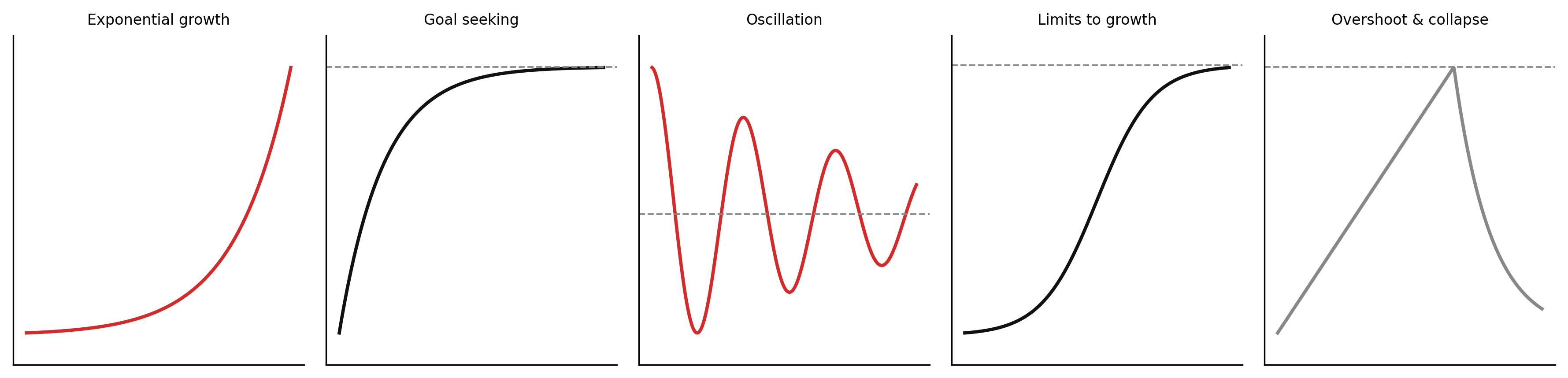
3.6 Delays in feedback loops
A delay is not simply a lag in the colloquial sense. In a stock-flow system, a delay is a stock — an intermediate accumulation that sits between a sensing point and a control point. Information or material must fill that stock before the signal reaches the regulator. Three kinds appear in practice.
A material delay is physical: hydrocarbon in transit between an injection point and a terminal cannot arrive instantaneously, regardless of how urgent the need. The pipeline itself is a delay stock. An information delay is the gap between a change in the real world and the point at which a decision-maker sees it: apportionment notices on a pipeline system propagate on monthly nomination cycles; a price signal must be observed, aggregated, and transmitted before it reaches a producer. A perception and response delay is the lag between receiving information and acting on it: a drilling programme takes eighteen to thirty-six months from investment decision to first barrel. Any realistic feedback loop contains at least one of these, and most contain all three in series.
The counterintuitive behaviour follows directly from the mechanism. In a balancing loop without delay, the corrective flow is proportional to the current gap between the stock and its goal. As the gap closes, the correction weakens. The system approaches the goal smoothly.
With a delay, the corrective flow is proportional to the gap as it was D time units ago — not as it is now. By the time the correction takes effect, the gap has already changed. Often it has reversed sign: the stock has already crossed the goal. The correction that was calibrated to the old gap is now excessive. It drives the stock past the goal in the other direction. A new corrective signal is generated, but it too arrives late. The result is oscillation around the goal, not convergence to it.
This is not a pathology of poorly designed systems. It is the mathematical consequence of inserting a stock between a sensing point and a control point. The longer the delay relative to the speed of correction, the wider the oscillation. If the delay is long enough, the oscillation does not dampen — the system becomes unstable.
The oil pipeline system from Chapter 1 runs two delays in series. Apportionment notices — the mechanism that communicates excess inventory to upstream nominators — propagate on monthly cycles. The drilling and completion programme that would increase supply operates on a horizon of one to three years: wells must be permitted, drilled, completed, and connected before a barrel moves. The balancing loop that connects a widening wellhead-to-export price spread to increased production volume exists, but its total delay is measured in years. During that interval, the reinforcing loops of investor expectation and speculative positioning can amplify the original imbalance rather than dampen it.
The data monitoring case is structurally identical. A deployed model’s performance begins to degrade — concept drift, distributional shift, upstream data quality changes. The time between when degradation begins and when a monitoring system detects it is an information delay embedded in the feedback loop between model performance and the retraining decision. A pipeline that batches evaluation metrics weekly and triggers retraining only after three consecutive failing evaluation windows may carry a total detection-to-response delay of several weeks. During that interval, the balancing loop that should correct the drift is not operating. The longer the monitoring lag, the wider the performance oscillation between retraining cycles.
The prescription that follows from recognising a delay is not to act faster — a faster correction through a delayed loop produces worse oscillation, not better. The prescription is either to shorten the delay or to reduce the aggressiveness of the correction.
NoteThe mathematics of delayed feedback
The behaviour described in this section — oscillation, damping, instability as a function of delay — has a formal mathematical treatment in control theory. Eigenvalues of the closed-loop system determine whether oscillations dampen or grow. Transfer functions in the Laplace domain make the delay explicit as a phase shift.
WH Maths Vol 8, Ch 1: Control, Feedback, and Stability develops this machinery in full, starting from the same thermostat example. If you want to know precisely why a gain of k and a delay of D produce instability when k × D exceeds a threshold, that is the place to go.
3.7 Simulating the thermostat: delay and oscillation
Exercise 2.3 asks you to trace the thermostat’s behaviour by hand under different delay assumptions; the code below runs those same assumptions across 240 minutes so the trajectories are visible at once. The three scenarios use identical parameters — same goal, same feedback gain, same starting temperature — and differ only in delay length, which is enough to produce three qualitatively distinct behaviours from the same balancing loop structure.
Code
"""Delayed thermostat — Chapter 2. Euler method with collections.deque delay buffer."""
import numpy as np
import matplotlib.pyplot as plt
from collections import deque

# Parameters
T_goal, T0, k, loss = 20.0, 15.0, 0.5, 0.05  # goal °C, start °C, gain, heat-loss rate
dt, t_end = 1.0, 240                           # Euler step (min), duration (min)
steps = int(t_end / dt) + 1
time  = np.arange(steps) * dt

# Three scenarios: (delay_minutes, colour, label)
scenarios = [
    ( 5, "#888888", "5-min delay"),
    (15, "#d52a2a", "15-min delay"),
    (45, "#111111", "45-min delay"),
]

fig, ax = plt.subplots(figsize=(8, 4), dpi=150)

for delay_min, color, label in scenarios:
    D_steps = int(delay_min / dt)                   # buffer length in time steps
    buf = deque([0.0] * D_steps, maxlen=D_steps)    # pre-fill: heater off at t=0

    T = np.empty(steps); T[0] = T0
    for i in range(steps - 1):
        gap       = T_goal - T[i]           # current sensing gap
        buf.append(k * gap)                 # store current control signal
        heating   = buf[0]                  # oldest (delayed) signal drives heater
        T[i + 1]  = T[i] + (heating - loss * T[i]) * dt

    ax.plot(time, T, color=color, linewidth=1.5, label=label)
    ax.annotate(label, xy=(240, T[-1]), fontsize=9, color=color, ha="right", va="center")

ax.axhline(y=T_goal, color="#888888", linestyle="--", linewidth=0.8)
ax.annotate("Goal (20°C)", xy=(5, T_goal), fontsize=8, color="#888888", va="bottom")

ax.set_xlim(0, 240)
ax.set_xlabel("Time (minutes)")
ax.set_ylabel("Room temperature (°C)")
ax.set_title("Thermostat with delay: three scenarios")
ax.spines["top"].set_visible(False)
ax.spines["right"].set_visible(False)
ax.grid(False)

plt.tight_layout()
plt.savefig("_assets/ch02-thermostat-simulation.png", dpi=150, bbox_inches="tight")
plt.show()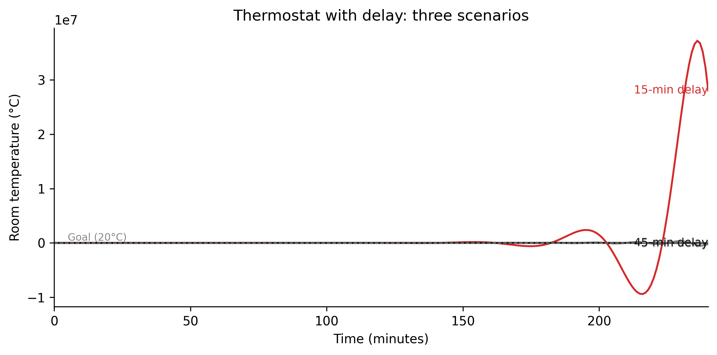
TipWhat to try
Increase the feedback strength (
k = 0.8) while keeping the 15-minute delay. What happens to the oscillation amplitude and frequency? Does stronger correction help or hurt?Set
loss = 0(a perfectly insulated room). How does this change the behaviour of the short-delay scenario? What does this tell you about the role of passive damping in stabilising a feedback loop?Match this to the pipeline system from Chapter 1. In that system, what plays the role of
T_goal,T0,k, andD? Write down the analogy explicitly — identify the stock, the goal, the feedback gain, and the two delays (apportionment cycle and drilling horizon) — before reading on.
import numpy as np
import matplotlib.pyplot as plt
from collections import deque

# --- Try changing these parameters ---
T_goal = 20.0   # Goal temperature (°C)
T0     = 15.0   # Starting temperature (°C)
k      = 0.5    # Feedback gain (try 0.8 to see stronger correction)
loss   = 0.05   # Heat-loss rate (try 0 for a perfectly insulated room)
t_end  = 240    # Duration (minutes)
dt     = 1.0    # Time step

scenarios = [
    ( 5, "#888888", "5-min delay"),
    (15, "#d52a2a", "15-min delay"),
    (45, "#111111", "45-min delay"),
]

steps = int(t_end / dt) + 1
time  = np.arange(steps) * dt

fig, ax = plt.subplots(figsize=(8, 4))
for delay_min, color, label in scenarios:
    D_steps = int(delay_min / dt)
    buf = deque([0.0] * D_steps, maxlen=D_steps)
    T = np.empty(steps); T[0] = T0
    for i in range(steps - 1):
        gap = T_goal - T[i]
        buf.append(k * gap)
        heating = buf[0]
        T[i + 1] = T[i] + (heating - loss * T[i]) * dt
    ax.plot(time, T, color=color, linewidth=1.5, label=label)
    ax.annotate(label, xy=(240, T[-1]), fontsize=9, color=color, ha="right", va="center")

ax.axhline(y=T_goal, color="#aaa", linestyle="--", linewidth=0.8)
ax.set_xlim(0, 240)
ax.set_xlabel("Time (minutes)")
ax.set_ylabel("Room temperature (°C)")
ax.set_title(f"Thermostat with delay  (k={k}, loss={loss})")
ax.spines["top"].set_visible(False)
ax.spines["right"].set_visible(False)
plt.tight_layout()
plt.show()
Figure 2.7. Room temperature over 240 minutes under three delay scenarios. With a short delay the balancing loop corrects smoothly. As delay increases, the loop overshoots its goal, generating oscillation. The 45-minute delay produces sustained cycling — the correction that was appropriate when initiated arrives after the system has already reversed direction.
3.8 Exercises
2.1 — Loop identification
For each of the following, identify whether the feedback loop is reinforcing or balancing, and draw a causal loop diagram:
- Wildfire: fire intensity → fuel consumption → available fuel → fire intensity
- Social proof: product popularity → recommendation to others → adoption → popularity
- Immune response: pathogen load → immune activation → pathogen clearance → pathogen load
- Traffic: congestion → route avoidance → reduced congestion
2.2 — Archetype matching
Match each of the following historical patterns to one of the five archetypes described above. Justify your answer with reference to the loop structure.
- The depletion of the Aral Sea (1960–2000)
- The adoption of smartphones (2007–2015)
- The US Federal Reserve’s interest rate adjustment in response to inflation
- The cod fishery collapse on the Grand Banks
2.3 — Archetype simulation
Implement a stock-flow model in Python for the “oscillation” archetype. Use a simple balancing loop with a delay:
- Stock: temperature of a room
- Goal: 20°C
- Delay: 15 minutes between heater activation and effect
- Run the simulation for 240 minutes, starting at 15°C
Plot the time series. What happens as you increase the delay? What happens as you increase the strength of the feedback?
2.4 — The ice-albedo feedback
The ice-albedo feedback is a reinforcing loop. But the Arctic has not experienced runaway warming — the feedback has not gone to its logical extreme. What balancing loops might be limiting the reinforcing feedback? Draw a causal loop diagram that shows both the reinforcing loop and at least two potential limiting mechanisms.
Krugman, Paul. 1991. “Increasing Returns and Economic Geography.” Journal of Political Economy 99 (3): 483–99. https://doi.org/10.1086/261763.
Meadows, Donella H. 2008. Thinking in Systems: A Primer. Chelsea Green Publishing.
Stroeve, Julienne C., Vladimir Kattsov, Andrew Barrett, et al. 2012. “Trends in Arctic Sea Ice Extent from CMIP5, CMIP3 and Observations.” Geophysical Research Letters 39 (16). https://doi.org/10.1029/2012GL052676.