flowchart LR
    DS(["Data Sources"])
    CD(["Consumed Data"])

    RDB[["Raw Data\nBacklog"]]
    PDS[["Processed\nData Stock"]]
    DQS[["Data Quality\nScore"]]

    DS  -->|"ingest rate\n(continuous)"| RDB
    RDB -->|"processing rate\n(capacity-limited)"| PDS
    PDS -->|"consumption"| CD
    RDB -->|"data issues"| DQS
    PDS -->|"monitoring +\nvalidation"| DQS

    style RDB fill:#fff3f3,stroke:#d52a2a,stroke-width:2px
    style PDS fill:#f5f5f5,stroke:#111111,stroke-width:2px
    style DQS fill:#f5f5f5,stroke:#111111,stroke-width:2px
    style DS  fill:#f5f5f5,stroke:#111111,stroke-width:2px
    style CD  fill:#f5f5f5,stroke:#111111,stroke-width:2px
7 Data as a System
Pipelines, feedback loops in machine learning, and the dynamics of concept drift
7.1 The puzzle
The spam filter trained on two years of labelled email data achieves 98% accuracy. Six months later, accuracy has fallen to 91%. No one changed the filter. No code was modified. No rules were altered. Email traffic is higher than ever. The filter is being tested on more data than it was trained on. It is failing on cases that look, to a human reviewer, like obvious spam.
The explanation is not a software bug. The spammers changed their vocabulary. The phrases that characterised spam in the training data — specific product names, phrasing patterns, URL formats — are no longer the phrases that characterise spam in the current data. The world drifted. The model stayed still.
This is concept drift: the phenomenon where the statistical relationship between inputs and outputs that a model learned from historical data no longer holds in the present. It is not a pathological edge case. It is the default condition for any model deployed into a world that continues to change after the training snapshot was taken.
The puzzle extends in both directions. Concept drift is the version where the world changes and the model doesn’t. But models also change the world they observe — through their own outputs. A recommendation model changes what users see. What users see changes what they click. What they click changes the training data for the next model iteration. A credit scoring model changes who gets loans. Who gets loans changes the loan repayment data that the next model is trained on. These feedback loops between model output and training data are not anomalies. They are structural features of any system where the model acts in the world it predicts.
This chapter applies the feedback structures from Chapters 1–5 to data systems directly. Data pipelines are stock-flow systems. Machine learning models sit inside feedback loops. Concept drift is what happens when a balancing loop is severed. Data quality is a stock that deteriorates without active maintenance. The mechanisms are the same. Only the material changes.
7.2 Data pipelines as stock-flow systems
Raw data is a stock. It accumulates through ingestion — sensor telemetry, user events, transactional records — and drains through processing. The ingest rate is typically continuous and externally driven: it depends on what is happening in the world, not on the processing system’s state. A sensor array generates readings at its sampling frequency regardless of whether the downstream pipeline is keeping pace. A web platform accumulates user events regardless of whether the ETL job has cleared yesterday’s batch. The processing rate is capacity-constrained. It cannot exceed what the infrastructure can handle. This asymmetry is the fundamental data engineering problem: ingest can always outpace throughput. When it does, the backlog accumulates.
An unprocessed data backlog is a stock in its own right. It accumulates when ingest exceeds processing capacity and drains when processing clears ahead. A growing backlog is not only a latency problem — it is a diagnostic signal that the inflow-outflow balance has been disrupted. Clearing a backlog requires running processing above its normal rate, which typically requires capacity investment: more compute, more parallel workers, more pipeline stages. The delay between the backlog accumulating and the capacity investment becoming operational is the same construction lag from Chapter 5. Housing supply cannot expand instantly. Processing capacity cannot expand instantly. The backlog persists during the delay. The longer the delay, the larger the backlog grows before the corrective capacity comes online.
Data quality does not remain constant over time. It deteriorates. Schema evolution in upstream systems introduces fields that parsers do not handle. Source systems change their encoding conventions without notifying downstream consumers. Sensor calibration coefficients drift as instruments age. Labels applied by human annotators two years ago no longer reflect current category definitions. Each of these is a flow draining the data quality stock. The balancing feedback that maintains quality is monitoring: automated checks detect quality failures, which trigger remediation, which restores quality. If monitoring is insufficient — too infrequent, too narrow in scope, too slow to produce an alert — the balancing loop is starved. Quality declines. The decline may be invisible for months because the degradation is gradual and no single failure is large enough to trigger an alert. By the time quality has fallen enough to be visible in downstream outputs, it has been deteriorating for an extended period.
The response timescale of a data quality issue depends on which stock is affected and how the failure mode propagates. A schema change that breaks a downstream parser fails immediately and visibly — the pipeline errors, the monitoring fires, the on-call engineer is paged within minutes. A gradual shift in a sensor’s calibration coefficient may not be detectable from any single record. It only appears as a statistical shift across thousands of records compared against an external reference. The same mismatch between fast inflows and slow detection that produces urban housing cycles produces data quality debt: by the time the problem is large enough to detect, it has been accumulating for months. The remediation cost at that point is larger than it would have been with earlier detection — exactly the committed damage structure from Chapter 4.
Earth domain: The GRACE data gap as feedback starvation
The GRACE satellite (Tapley et al. 2004) measured terrestrial water storage and ice mass through gravity anomalies. It was decommissioned in October 2017. Its replacement, GRACE-FO, launched in May 2018. The 11-month gap between them severed the feedback loop between observed ice mass change and Earth system models that used GRACE data as a forcing or validation input. Models continued running during the gap. Their outputs drifted from the true system state at a rate proportional to the unobserved change in Greenland and Antarctic mass balance. The gap is the data engineering version of committed warming from Chapter 4: future model error was locked in during the period when the feedback loop was severed, regardless of what happened after GRACE-FO data became available. The backlog of unobserved Earth system state cannot be recovered retrospectively. The stock evolved; the observation did not.
Data domain: A production ML pipeline as a multi-stock system
A production ML pipeline contains three primary stocks: raw features (upstream data, continuously generated), trained model weights (updated on a schedule), and model performance metrics (measured continuously against held-out data or live outcomes). Three flows connect them: feature ingestion fills the raw features stock, training runs consume raw features and update model weights, and performance evaluation measures the gap between model state and current world state. The delays between these flows determine the system’s response time to concept drift. A model retrained monthly will lag a world that changes weekly by a gap that grows throughout each retraining interval. The delay structure of the pipeline determines the worst-case accuracy degradation that can accumulate before the next corrective action.
The stock-flow structure here is diagnostic. When model accuracy falls, the question is not “what is wrong with the model?” The question is: which stock has deteriorated, which flow is insufficient, and what delay is preventing the corrective loop from operating at the required frequency?
Diagram 6.1 shows the stock-flow structure of a production data pipeline: the raw data backlog, the processed data stock, and the data quality stock, with ingest and processing flows and the monitoring balancing loop that maintains quality.
Figure 6.1. Data pipeline as a stock-flow system. The raw data backlog accumulates when ingest rate exceeds processing capacity — the same asymmetric inflow/outflow structure as urban housing shortage. Data quality is a separate stock maintained by the balancing feedback of monitoring and validation; without active monitoring, quality decays through schema drift and sensor calibration errors. The three stocks have different response timescales: backlog responds to throughput changes in hours; processed data stock responds in days; data quality degradation may be invisible for months.
NotePipeline architecture and data quality monitoring
The stock-flow structure described here — raw data, processing capacity, backlog, data quality — has a direct engineering counterpart in production data systems. Schema validation, data lineage tracking, anomaly detection on feature distributions, and SLA monitoring are the engineering instruments that keep the balancing loops operational.
WH Data Engineering Ch 3 (Pipelines and ETL) and Ch 7 (Governance) covers the specific tools and architectural patterns — dbt, Great Expectations, Apache Airflow — that implement these monitoring loops. This chapter provides the systems thinking framework; Data Engineering provides the implementation.
7.3 Feedback loops in machine learning
A deployed model is not an isolated system. It acts in the world. Its actions change the world. The changed world generates new data. The new data becomes the training signal for the next model iteration. This chain is a feedback loop, and its properties — reinforcing or balancing, fast or slow, stable or oscillating — determine the long-run behaviour of the model as much as its architecture or training procedure.
Three loop types appear consistently in production ML systems.
Loop 1: The retraining balancing loop (the intended design). The intended architecture of a production ML system is a balancing loop. The model makes predictions. Some fraction of those predictions can be verified against observed outcomes. The gap between predicted and observed — the error — drives retraining. Retraining reduces error. A smaller error generates less retraining signal. The loop seeks a goal state: minimum prediction error on the current data distribution.
This is a goal-seeking feedback structure — identical to the thermostat from Chapter 2. The goal is zero prediction error on the current distribution. The corrective action is retraining. The delays are labelling latency (how long before outcomes can be observed and labelled), retraining cost (compute and time required to retrain), and deployment cycle (time between a retrained model being ready and its deployment in production). Long delays in this loop produce the same oscillation and lag that delays produce in any balancing system. The model that was optimal at training time arrives in production weeks or months later into a world that has continued to change during the delay.
Loop 2: Reinforcing degradation through distribution shift. When the retraining balancing loop is too slow — when concept drift accumulates faster than retraining clears it — a secondary reinforcing loop can activate. Model accuracy falls. Users begin to distrust or ignore model outputs. Feedback from users (clicks, corrections, explicit labels) declines in volume or quality. The training signal weakens. Less retraining signal means less effective retraining. Less effective retraining means accuracy continues to fall. The loop is reinforcing in the downward direction: accuracy decline → weaker feedback → less retraining → further accuracy decline.
This is the Detroit inversion from Chapter 5 applied to ML systems. The same mechanism that produces urban disinvestment cascades produces model degradation cascades. The feedback starvation that allows this loop to activate is structural: if the monitoring and retraining infrastructure is not built, the balancing loop does not exist, and the reinforcing loop operates unchecked.
Loop 3: The filter bubble — reinforcing constriction. In recommendation systems, the deployed model produces training data for its own successor. The model recommends content. Users engage with the recommended content. The engagement record becomes training data labelled as “relevant.” The next model iteration learns that what was recommended was relevant — because relevance was measured by engagement with recommendations, not by independent assessment of the content space. The loop: model recommends narrowly → users engage with narrow content → narrow engagement record → next model trained to recommend narrowly. The distribution of recommended content constricts over time, not because users prefer narrower content, but because the feedback loop measures engagement with what was shown, not preferences across what was not shown.
Human domain: Credit scoring during COVID-19
Credit scoring models trained on pre-2020 repayment behaviour were built on the assumption that the economic conditions generating repayment signals would remain approximately stable (Sculley et al. 2015). COVID-19 violated that assumption instantaneously. Unemployment rates spiked. Government transfer payments replaced earned income. Loan forbearance programmes suspended normal repayment signals. The features that predicted default in the training data — missed payments, income instability — were being triggered by a government policy response rather than by creditworthiness in the traditional sense. Banks that continued using pre-pandemic models for credit decisions were running the spam filter scenario at enormous scale: the world had changed, the models had not, and the gap between the two was growing.
Earth domain: Land cover classifier drift
A Landsat-based land cover classifier trained on data from 2000–2010 will misclassify shrub expansion into tundra as warming drives it northward in the 2020s. The spectral signatures of shrub-covered tundra and grass-covered tundra were distinguishable in the training period. The proportions of those classes at high latitudes were approximately stable. By 2025, the Arctic is measurably different from what the model was trained on. The classifier’s confusion matrix for Arctic pixels has drifted. The model is not wrong about the 2000–2010 Arctic. It is wrong about the 2025 Arctic, and the drift is accelerating.
Diagram 6.2 shows the retraining balancing loop: how prediction error drives retraining signal through labelling latency delays to update model weights and reduce error.
graph LR
    MA["Model\nAccuracy"]
    PE["Prediction\nError"]
    RS["Retraining\nSignal"]
    LL["Labelling\nLatency"]
    TR["Training\nRun"]
    MW["Model\nWeights"]
    CD["Concept\nDrift"]

    MA -->|"−"| PE
    PE -->|"+"| RS
    RS -->|"+"| LL
    LL -->|"+"| TR
    TR -->|"+"| MW
    MW -->|"+ [B]"| MA
    CD -->|"−"| MA

    style MA fill:#fff3f3,stroke:#d52a2a,stroke-width:2px
    style PE fill:#f5f5f5,stroke:#111111,stroke-width:2px
    style RS fill:#f5f5f5,stroke:#111111,stroke-width:2px
    style LL fill:#f5f5f5,stroke:#111111,stroke-width:2px
    style TR fill:#f5f5f5,stroke:#111111,stroke-width:2px
    style MW fill:#f5f5f5,stroke:#111111,stroke-width:2px
    style CD fill:#f5f5f5,stroke:#111111,stroke-width:2px
Figure 6.2. ML retraining as a balancing feedback loop. Prediction error drives a retraining signal, which (after labelling latency and training cost delays) updates model weights and reduces error. Concept drift is the external stress that continuously pushes accuracy downward, competing against the corrective retraining flow. The loop’s ability to maintain accuracy depends on whether the retraining rate exceeds the drift rate — a direct application of the disturbance-vs-correction rate comparison from Chapter 2.
Diagram 6.3 shows the reinforcing degradation loop: how accuracy decline starves user feedback, weakening training data quality and retraining effectiveness in a self-amplifying collapse.
graph LR
    MA["Model\nAccuracy"]
    UT["User\nTrust"]
    UFV["User\nFeedback\nVolume"]
    TDQ["Training\nData\nQuality"]
    RE["Retraining\nEffectiveness"]
    CD["Concept\nDrift"]

    MA  -->|"+"| UT
    UT  -->|"+"| UFV
    UFV -->|"+"| TDQ
    TDQ -->|"+"| RE
    RE  -->|"+ [R]"| MA
    CD  -->|"−"| MA

    style MA  fill:#fff3f3,stroke:#d52a2a,stroke-width:2px
    style UT  fill:#f5f5f5,stroke:#111111,stroke-width:2px
    style UFV fill:#f5f5f5,stroke:#111111,stroke-width:2px
    style TDQ fill:#f5f5f5,stroke:#111111,stroke-width:2px
    style RE  fill:#f5f5f5,stroke:#111111,stroke-width:2px
    style CD  fill:#f5f5f5,stroke:#111111,stroke-width:2px
Figure 6.3. Concept drift reinforcing degradation loop. When accuracy falls, users trust the model less and provide less feedback. Less feedback degrades training data quality. Poorer training data reduces the effectiveness of each retraining cycle. Lower retraining effectiveness allows accuracy to fall further. Zero − signs in the main loop → reinforcing (R). This is the Detroit inversion from Chapter 5 applied to ML systems: the same mechanism that makes a platform valuable when accuracy is high makes it collapse rapidly when accuracy falls past a threshold.
Diagram 6.4 shows the filter bubble reinforcing loop: how recommendation outputs become training inputs, progressively concentrating the content distribution regardless of true user preferences.
graph LR
    RN["Recommendation\nNarrowness"]
    UE["User Engagement\nWith Narrow\nContent"]
    TSN["Training Signal\nNarrowness"]
    MCB["Model\nContent Bias"]
    UPD["User Preference\nDiversity"]

    RN  -->|"+"| UE
    UE  -->|"+"| TSN
    TSN -->|"+"| MCB
    MCB -->|"+ [R]"| RN
    UPD -->|"−"| RN

    style RN  fill:#fff3f3,stroke:#d52a2a,stroke-width:2px
    style UE  fill:#f5f5f5,stroke:#111111,stroke-width:2px
    style TSN fill:#f5f5f5,stroke:#111111,stroke-width:2px
    style MCB fill:#f5f5f5,stroke:#111111,stroke-width:2px
    style UPD fill:#f5f5f5,stroke:#111111,stroke-width:2px
Figure 6.4. Filter bubble reinforcing loop. Recommendations narrow user engagement, which narrows training signals, which increases model content bias, which narrows recommendations further. Zero − signs in the main loop → reinforcing (R). The critical structural flaw: user preference diversity (what users would prefer if shown a wider selection) is not in the feedback loop — it is measured only indirectly through engagement with what was already recommended. The loop amplifies its own training signal rather than learning from the full preference distribution.
7.4 Loss landscapes as energy landscapes
Gradient descent is a feedback loop. The model makes predictions. The predictions are compared to labels. The discrepancy is the loss. The gradient of the loss with respect to the model parameters points in the direction of increasing loss. The update rule moves the parameters in the opposite direction. The loop: high loss → gradient signal → parameter update → reduced loss. This is a balancing loop: the loss is the discrepancy from the goal state of zero error, and the gradient is the corrective action.
The loss landscape is the energy landscape of this feedback system. A convex loss landscape has a single basin — one attractor. The balancing loop reliably converges to the global minimum regardless of starting point. A non-convex loss landscape has multiple basins — multiple local minima. The balancing loop converges to whichever minimum is nearest to the starting point. The model that gradient descent finds is determined not only by the data but by the initialisation and the path taken through parameter space. This is path dependence in loss space: the same mechanism that determines which city wins in the two-city simulation from Chapter 5. The attractor the system reaches depends on where it started, not just on the shape of the landscape.
The learning rate is the parameter that controls the strength of the corrective action. Too low: convergence is slow, and the model may stop improving before reaching the minimum, stalling in a flat region. Too high: the update overshoots the minimum, and the model oscillates or diverges. This is the same delay-and-gain trade-off that governs any balancing feedback system. The right learning rate is the one that produces goal-seeking convergence without overshoot — the same design criterion as a well-tuned thermostat or a well-calibrated policy response in any stock-flow system. Learning rate is the gain of the gradient descent feedback loop.
NoteGradient descent as a dynamical system
The connection between gradient descent and dynamical systems is exact, not metaphorical. Gradient flow — the continuous-time limit of gradient descent — is a differential equation of the form dx/dt = −∇L(x), where L is the loss function. The fixed points of this equation are the critical points of the loss: minima, maxima, and saddle points. Stability of a critical point is determined by the eigenvalues of the Hessian at that point — exactly the linear stability analysis from the climate sensitivity section of Chapter 4.
WH Maths Vol 8, Ch 1 (Control, Feedback, Stability) develops the connection between gradient flow and control theory: the loss landscape is the Lyapunov function, and convergence is guaranteed when the loss is strongly convex. Non-convex landscapes — the norm in deep learning — are where the analogy with tipping points from Chapter 3 becomes relevant.
7.5 Concept drift — the balancing loop severed
Concept drift is the structural condition where the statistical distribution the model was trained on diverges from the distribution on which it is being evaluated. Three mechanisms produce it.
Data drift — the input distribution changes. The kinds of inputs arriving at the model change in frequency or character: different spam vocabulary, different user demographics, different sensor reading ranges as climate changes. The model has not changed. The world feeding it has.
Label drift — the mapping from inputs to outputs changes. The same input now corresponds to a different correct label: a phrase that was not spam in 2022 is spam in 2024 because its use has been adopted by spammers. The feature space is the same. The target function has moved.
Prior drift — the base rate of the target variable changes. Fraud was 0.1% of transactions in 2019; it was 0.4% of transactions in 2021 because the COVID-19 period enabled new fraud vectors. A model calibrated to a 0.1% prior is miscalibrated. Its decision threshold, set to be optimal at the training-time prior, generates too many false negatives at the current prior.
All three produce the same system-level symptom: the balancing retraining loop, which should keep model accuracy near its goal state, is operating against a shifting target. If the target moves faster than the loop can follow, accuracy degrades continuously. The severity depends on the ratio of drift rate to retraining frequency — the same ratio of disturbance rate to corrective response rate that determines whether any balancing loop stays near its goal.
The detection problem is as important as the correction problem. Concept drift is often invisible until it has accumulated to a detectable threshold — by which point, the model has been wrong at scale for an extended period. Early detection requires monitoring the input distribution, not only model performance. Tracking feature statistics over time and comparing current data distributions to training distributions places the monitoring upstream of the accuracy degradation in the causal chain. A monitoring system that only measures model accuracy will detect drift late, after the accuracy has already fallen. A monitoring system that measures input distributions will detect drift early — distribution shift precedes accuracy degradation causally, because the distribution must shift before the predictions degrade. The detection delay that separates early from late monitoring is a delay in the balancing loop: shorter delay, faster correction, smaller total accuracy loss.
Data domain: EO classifier retraining in a changing Arctic
A cryosphere classification model monitoring permafrost extent from Sentinel-1 SAR data faces accelerating concept drift. The permafrost extent it was trained to classify is shrinking. New terrain types are appearing — thermokarst lakes, subsided tundra, drainage channels — that were rare or absent in the training data. Retraining requires new field validation data from these novel terrain types, which requires field campaigns in remote Arctic locations. The retraining loop is slow: field campaign planning, data collection, model retraining, validation, and deployment takes 18–24 months. The drift rate may be faster. This is a case where the balancing loop — retraining — cannot keep pace with the disturbance rate, and the model’s concept of “permafrost” diverges from the current Arctic faster than it can be corrected.
NoteConcept drift in Earth observation classifiers
The phenomena described here — Arctic land cover change, permafrost thaw, vegetation encroachment — appear in WH Computational Geography Parts 2 and 4 (Earth Observation and Hazards) as classification and change detection problems. The computational geography treatment covers the specific remote sensing techniques for detecting these changes. This chapter explains why classifiers trained on historical data fail to detect them: the training distribution and the current distribution have diverged, and the retraining loop cannot keep pace with the rate of change.
7.6 Simulating the retraining loop under concept drift
The model below simulates the retraining balancing loop under concept drift. Model accuracy is a stock that drifts downward as the world changes. Retraining raises it — but with a delay, and only to the extent that fresh training data is available. Three scenarios run in parallel: no retraining (accuracy drifts to floor), periodic retraining (accuracy oscillates around a degraded mean), and adaptive retraining triggered by a threshold (accuracy stabilises near the goal). The key result: the adaptive loop outperforms periodic retraining not because it retrains more often on average, but because it retrains at the right time — when the accuracy gap is largest. Periodic retraining that fires on a schedule may retrain when drift is minimal and miss the window when drift is accelerating. Threshold-triggered retraining acts proportionally to the discrepancy, which is the design of any well-functioning balancing feedback loop.
Code
"""ML retraining loop under concept drift — Chapter 6.
Euler integration of two stocks: model accuracy and training data freshness.
Three scenarios: no retraining, periodic fixed-schedule, adaptive threshold-triggered."""
import numpy as np
import matplotlib.pyplot as plt

# -- Named constants -----------------------------------------------------------
ACCURACY_FLOOR     = 0.50   # random-chance baseline for binary classification
ACCURACY_CEILING   = 0.95   # best achievable accuracy with perfectly fresh data
ACCURACY_THRESHOLD = 0.80   # adaptive trigger: retrain when accuracy falls below this
D                  = 0.08   # drift rate (per year)
RETRAIN_PERIOD     = 1.0    # fixed-schedule retraining interval (years)
MIN_RETRAIN_GAP    = 0.25   # minimum time between retraining events (years, adaptive)
DT                 = 0.01   # Euler time-step (years)
T_START            = 0.0
T_END              = 10.0

# WH palette
COL_NONE     = "#888888"    # no retraining
COL_PERIODIC = "#111111"    # periodic retraining
COL_ADAPTIVE = "#d52a2a"    # adaptive retraining


# -- Euler simulation ----------------------------------------------------------
def run_simulation(retrain_policy):
    """
    Run one 10-year Euler simulation.
    retrain_policy: one of 'none', 'periodic', 'adaptive'
    Returns: (t, accuracy, freshness, retrain_times)
    """
    steps         = int((T_END - T_START) / DT) + 1
    t             = np.linspace(T_START, T_END, steps)
    accuracy      = np.empty(steps)
    freshness     = np.empty(steps)
    retrain_times = []

    # Initial conditions: well-trained model, perfectly fresh data
    accuracy[0]  = ACCURACY_CEILING
    freshness[0] = 1.0
    last_retrain = -999.0   # track time of last retraining event

    for i in range(1, steps):
        t_now = t[i]

        # -- Decay stocks via Euler step ----------------------------------------
        acc_prev   = accuracy[i - 1]
        fresh_prev = freshness[i - 1]

        # Accuracy decays exponentially toward the floor (concept drift)
        d_accuracy  = -D * (acc_prev - ACCURACY_FLOOR)
        # Data freshness decays exponentially toward zero (world changes)
        d_freshness = -D * fresh_prev

        acc_new   = acc_prev   + d_accuracy  * DT
        fresh_new = fresh_prev + d_freshness * DT

        # -- Check for a retraining event this step ----------------------------
        retrain_now = False

        if retrain_policy == "periodic":
            # Detect crossing of a schedule boundary inside this step
            prev_interval = (t[i - 1] - T_START) / RETRAIN_PERIOD
            curr_interval = (t_now    - T_START) / RETRAIN_PERIOD
            if int(curr_interval) > int(prev_interval):
                retrain_now = True

        elif retrain_policy == "adaptive":
            # Retrain when accuracy falls below threshold, subject to minimum gap
            elapsed_since_last = t_now - last_retrain
            if acc_new < ACCURACY_THRESHOLD and elapsed_since_last >= MIN_RETRAIN_GAP:
                retrain_now = True

        # -- Apply retraining effects ------------------------------------------
        if retrain_now:
            # Accuracy is restored in proportion to how fresh the training data is
            acc_new   = ACCURACY_FLOOR + (ACCURACY_CEILING - ACCURACY_FLOOR) * fresh_new
            # Data freshness is fully restored by ingesting new labels
            fresh_new = 1.0
            last_retrain = t_now
            retrain_times.append(t_now)

        accuracy[i]  = acc_new
        freshness[i] = fresh_new

    return t, accuracy, freshness, retrain_times


# -- Run all three scenarios ---------------------------------------------------
t0, acc0, fresh0, rt0 = run_simulation("none")
t1, acc1, fresh1, rt1 = run_simulation("periodic")
t2, acc2, fresh2, rt2 = run_simulation("adaptive")


# -- Figure: 2 panels ----------------------------------------------------------
fig, (ax1, ax2) = plt.subplots(2, 1, figsize=(10, 7), dpi=150)

# -- Panel 1: Model accuracy ---------------------------------------------------
ax1.plot(t0, acc0, color=COL_NONE,     linestyle="--", linewidth=1.2)
ax1.plot(t1, acc1, color=COL_PERIODIC, linestyle="-",  linewidth=1.8)
ax1.plot(t2, acc2, color=COL_ADAPTIVE, linestyle="-",  linewidth=1.8)

# Reference line at accuracy threshold
ax1.axhline(ACCURACY_THRESHOLD, color="#888888", linestyle="--",
            linewidth=0.7, zorder=0)
ax1.annotate("Threshold 0.80", xy=(0.12, ACCURACY_THRESHOLD),
             xytext=(0.12, ACCURACY_THRESHOLD + 0.015),
             fontsize=8, color="#888888", va="bottom")

# Annotate scenario lines at right edge
label_offsets = {"No retraining": -0.03, "Periodic": 0.02, "Adaptive": 0.02}
for label, t_, acc_, col in [
    ("No retraining", t0, acc0, COL_NONE),
    ("Periodic",      t1, acc1, COL_PERIODIC),
    ("Adaptive",      t2, acc2, COL_ADAPTIVE),
]:
    ax1.annotate(label,
                 xy=(t_[-1], acc_[-1]),
                 xytext=(t_[-1] - 0.1, acc_[-1] + label_offsets[label]),
                 fontsize=8.5, color=col, ha="right", va="center")

ax1.set_xlim(T_START, T_END)
ax1.set_ylim(0.40, 1.02)
ax1.set_ylabel("Model accuracy")
ax1.spines["top"].set_visible(False)
ax1.spines["right"].set_visible(False)
ax1.grid(False)

# -- Panel 2: Training data freshness ------------------------------------------
ax2.plot(t0, fresh0, color=COL_NONE,     linestyle="--", linewidth=1.2)
ax2.plot(t1, fresh1, color=COL_PERIODIC, linestyle="-",  linewidth=1.8)
ax2.plot(t2, fresh2, color=COL_ADAPTIVE, linestyle="-",  linewidth=1.8)

# Mark retraining events as faint vertical ticks
for rt in rt1:
    ax2.axvline(rt, color=COL_PERIODIC, alpha=0.3, linewidth=0.8)
for rt in rt2:
    ax2.axvline(rt, color=COL_ADAPTIVE, alpha=0.3, linewidth=0.8)

# Annotate scenario lines at right edge
fresh_offsets = {"No retraining": -0.04, "Periodic": 0.03, "Adaptive": 0.03}
for label, t_, fresh_, col in [
    ("No retraining", t0, fresh0, COL_NONE),
    ("Periodic",      t1, fresh1, COL_PERIODIC),
    ("Adaptive",      t2, fresh2, COL_ADAPTIVE),
]:
    ax2.annotate(label,
                 xy=(t_[-1], fresh_[-1]),
                 xytext=(t_[-1] - 0.1, fresh_[-1] + fresh_offsets[label]),
                 fontsize=8.5, color=col, ha="right", va="center")

ax2.set_xlim(T_START, T_END)
ax2.set_ylim(-0.05, 1.10)
ax2.set_xlabel("Year")
ax2.set_ylabel("Training data freshness")
ax2.spines["top"].set_visible(False)
ax2.spines["right"].set_visible(False)
ax2.grid(False)

plt.tight_layout(pad=1.5)
plt.savefig("_assets/ch06-concept-drift.png", dpi=150, bbox_inches="tight")
plt.show()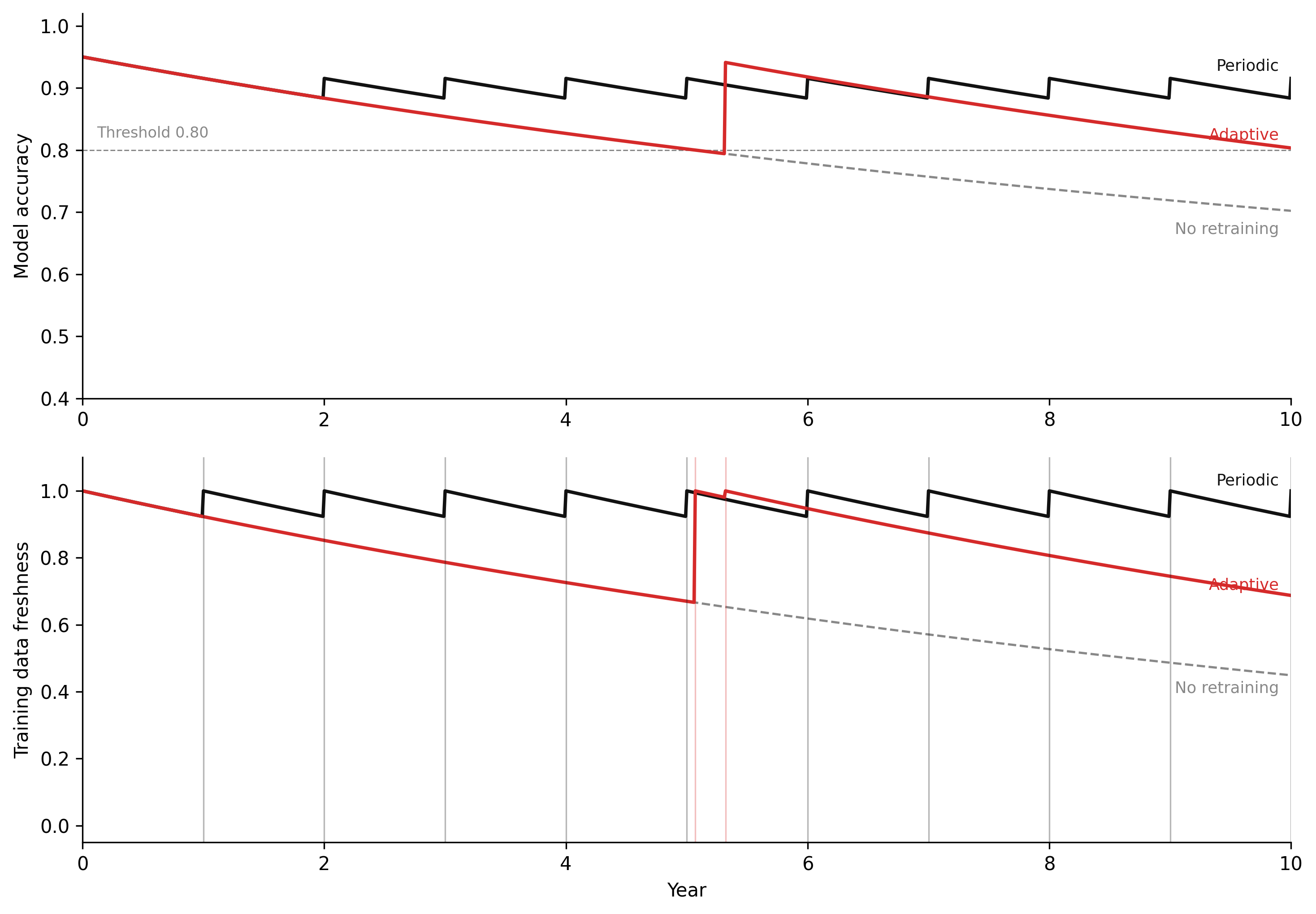
TipWhat to try
Double the drift rate (
D = 0.16). How does this affect the performance of periodic retraining? How frequently would periodic retraining need to occur to maintain accuracy above 0.80? What does this imply about system design in rapidly changing environments — for example, a fraud detection model facing a novel attack campaign where the attacker adapts faster than the retraining cycle?Increase the retraining threshold to 0.88. How does this change the retraining frequency in Scenario 2? Is the mean accuracy over the 10-year period higher or lower than with
ACCURACY_THRESHOLD = 0.80? Does more frequent retraining always improve average performance, or does the freshness penalty from triggering early cut into gains?Simulate data freshness decay with a labelling lag. Add a 0.25-year lag: when the accuracy threshold is crossed,
data_freshnesscontinues to decay for 0.25 years before the retrain executes. How much does this delay degrade the post-retrain accuracy ceiling compared to instantaneous retraining, and does the gap widen or stay constant across the 10-year window?
import numpy as np
import matplotlib.pyplot as plt

# --- Try changing these parameters ---
D                  = 0.08   # drift rate per year (try 0.16 for rapid drift)
RETRAIN_PERIOD     = 1.0    # periodic retraining interval in years
ACCURACY_THRESHOLD = 0.80   # adaptive trigger threshold (try 0.88)
LABELLING_LAG      = 0.0    # delay before retrain executes after threshold crossed (try 0.25)

ACCURACY_FLOOR    = 0.50
ACCURACY_CEILING  = 0.95
MIN_RETRAIN_GAP   = 0.25
DT = 0.01
T_START, T_END = 0.0, 10.0
steps = int((T_END - T_START) / DT) + 1
t = np.linspace(T_START, T_END, steps)

def run(policy):
    acc = np.empty(steps); fresh = np.empty(steps)
    acc[0] = ACCURACY_CEILING; fresh[0] = 1.0
    last_retrain = -999.0; lag_triggered_at = None
    for i in range(1, steps):
        d_acc   = -D * (acc[i-1]   - ACCURACY_FLOOR)
        d_fresh = -D * fresh[i-1]
        acc[i]   = acc[i-1]   + d_acc   * DT
        fresh[i] = fresh[i-1] + d_fresh * DT
        retrain_now = False
        if policy == "periodic":
            if int((t[i] - T_START) / RETRAIN_PERIOD) > int((t[i-1] - T_START) / RETRAIN_PERIOD):
                retrain_now = True
        elif policy == "adaptive":
            if lag_triggered_at is None and acc[i] < ACCURACY_THRESHOLD and (t[i] - last_retrain) >= MIN_RETRAIN_GAP:
                lag_triggered_at = t[i]
            if lag_triggered_at is not None and (t[i] - lag_triggered_at) >= LABELLING_LAG:
                retrain_now = True; lag_triggered_at = None
        if retrain_now:
            acc[i]   = ACCURACY_FLOOR + (ACCURACY_CEILING - ACCURACY_FLOOR) * fresh[i]
            fresh[i] = 1.0
            last_retrain = t[i]
    return acc, fresh

acc0, fresh0 = run("none")
acc1, fresh1 = run("periodic")
acc2, fresh2 = run("adaptive")

fig, (ax1, ax2) = plt.subplots(2, 1, figsize=(9, 6))
ax1.plot(t, acc0, color="#888", linestyle="--", linewidth=1.2, label="No retraining")
ax1.plot(t, acc1, color="#111", linewidth=1.6, label=f"Periodic ({RETRAIN_PERIOD} yr)")
ax1.plot(t, acc2, color="#d52a2a", linewidth=1.6, label=f"Adaptive (threshold={ACCURACY_THRESHOLD})")
ax1.axhline(ACCURACY_THRESHOLD, color="#aaa", linestyle="--", linewidth=0.7)
ax1.set_ylabel("Model accuracy"); ax1.set_xlim(T_START, T_END); ax1.set_ylim(0.4, 1.02)
ax1.legend(frameon=False, fontsize=9)
ax1.spines["top"].set_visible(False); ax1.spines["right"].set_visible(False)

ax2.plot(t, fresh0, color="#888", linestyle="--", linewidth=1.2)
ax2.plot(t, fresh1, color="#111", linewidth=1.6)
ax2.plot(t, fresh2, color="#d52a2a", linewidth=1.6)
ax2.set_xlabel("Year"); ax2.set_ylabel("Training data freshness")
ax2.set_xlim(T_START, T_END); ax2.set_ylim(-0.05, 1.1)
ax2.spines["top"].set_visible(False); ax2.spines["right"].set_visible(False)

plt.tight_layout()
plt.show()
Figure 6.5. ML retraining loop under concept drift across three retraining policies (D = 0.08 per year, accuracy floor = 0.50, accuracy ceiling = 0.95). Top panel: model accuracy over 10 years. Without retraining (grey dashed), accuracy decays exponentially toward random-chance baseline. Periodic retraining (black) produces a regular sawtooth — accuracy recovers fully after each event but always decays again on the same schedule regardless of how fast the world is drifting. Adaptive retraining (red) holds accuracy above the 0.80 threshold with events spaced by actual need. Bottom panel: training data freshness with retraining events as faint vertical ticks. The vertical ticks reveal that adaptive retraining fires less often than the fixed schedule when drift is slow — the policy is more efficient, not just faster.
7.7 Exercises
6.1 — Data pipeline stock-flow
A production data pipeline ingests sensor data at 10,000 records/hour. The processing system has a validated throughput capacity of 8,000 records/hour. Processing takes the raw records through three stages: validation, enrichment, and aggregation.
- Draw the stock-flow diagram for this pipeline. Identify the backlog stock and all relevant flows. What is the net accumulation rate of the backlog under current conditions?
- The processing capacity can be doubled by adding parallel processing workers, but requires 6 weeks of infrastructure work to deploy. Sketch the time series of backlog size over the next 6 months under the assumption that the expansion proceeds. What archetype from Chapter 2 describes this trajectory?
- A naive solution is to lower validation strictness to increase throughput. Which flow does this intervention affect, and what stock does it deteriorate? Why might this intervention make the long-run problem worse even though it solves the short-run backlog?
6.2 — ML retraining loop
A fraud detection model is deployed in a payments system. The model produces scores for each transaction. Transactions flagged as high-risk are reviewed by human analysts, who confirm or correct the model’s label. Confirmed fraud cases and corrected non-fraud cases become training data for the next model version. The model is retrained every 90 days.
- Draw the full causal loop diagram for this system. Identify the retraining balancing loop and all delays within it.
- Fraud tactics evolve on a roughly 30-day cycle: after a new attack pattern is flagged and blocked, fraudsters adapt. What does this imply about the 90-day retraining frequency relative to the drift rate? Describe the expected accuracy trajectory over a 12-month period under current conditions.
- The fraud operations team proposes reducing the retraining cycle to 30 days. What new risks does this introduce? Identify the specific feedback loops and stocks affected by higher retraining frequency.
6.3 — Filter bubble loop analysis
A video recommendation platform trains its model on user engagement data. A user who watches one political commentary video is subsequently shown more videos with similar content. The user’s watch history becomes progressively more concentrated in that content category over 6 months.
- Draw the full causal loop diagram showing how the recommendation loop produces content concentration. Label every link and every loop as R or B.
- The platform introduces a “diversity injection” mechanism: 10% of recommendations are randomly selected from outside the user’s current content cluster. Which link in your diagram does this intervention modify? Is the loop structure R or B after the intervention?
- Propose a metric that would allow the platform to detect filter bubble formation before users notice it. Describe: (i) what it measures, (ii) how it would change over time in the presence and absence of a filter bubble, and (iii) what threshold would trigger an intervention.
6.4 — Concept drift detection
A sentiment analysis model is trained on product reviews from 2019–2021. It is deployed to monitor brand sentiment in 2023.
- List three specific mechanisms by which concept drift could affect this model between 2021 and 2023. For each, identify whether it is data drift, label drift, or prior drift.
- The monitoring team measures model accuracy weekly using a sample of human-labelled reviews. Accuracy appears stable for 8 months, then drops 12% in 6 weeks. Propose a causal explanation for this sudden drop that is consistent with gradual concept drift accumulating over 8 months before becoming visible in accuracy metrics.
- Redesign the monitoring system to detect drift earlier. What additional metrics, beyond model accuracy, would you track? How does each metric connect to the causal chain between world change and model failure?
6.5 — Loss landscape and learning rate
A neural network is being trained on a classification task. The loss landscape in the neighbourhood of the current parameters has the following properties: convex in one direction (corresponding to the primary feature) and nearly flat in another direction (corresponding to a feature with low predictive value).
- Sketch the expected trajectory of gradient descent in this landscape for (i) a learning rate that is too high, (ii) a learning rate that is too low, and (iii) an approximately optimal learning rate. For each, describe the corresponding behaviour of the loss over training iterations.
- The flat direction of the landscape corresponds to a feature that has low predictive value in the training data but high predictive value for the actual deployment task (a domain shift). How does the gradient descent update rule handle this — and what does this imply about the model’s ability to perform well on the deployment task?
- Connect this scenario to the concept drift framework. The flat landscape direction corresponds to a feature the model has not learned. When the deployment distribution shifts to make that feature important, what happens to the accuracy trajectory? What would retraining on the new distribution require?
6.6 — System design for resilience
You are designing the monitoring and retraining infrastructure for a land cover classification model deployed in a wildfire risk assessment system in western Canada. The model classifies vegetation type from Sentinel-2 imagery. Wildfire risk scores for specific locations are downstream outputs.
- Identify three feedback loops that this system depends on to remain accurate over time. For each loop, identify: the stock being maintained, the corrective flow, and the delay.
- Identify the most critical single point of feedback starvation in this system — the severing of which loop would most rapidly degrade the risk assessment outputs. Justify your choice.
- Design a monitoring protocol that would detect feedback starvation in your identified critical loop before it causes visible accuracy degradation. Specify: monitoring frequency, the specific distribution or metric being tracked, the threshold for escalation, and the escalation action.
- In 2024, the Canadian Forest Service substantially changes its vegetation classification schema to include additional shrub subcategories. Identify which type of concept drift this represents and describe the expected impact on the wildfire risk model’s outputs if no retraining occurs within 12 months.
Sculley, D., Gary Holt, Daniel Golovin, et al. 2015. “Hidden Technical Debt in Machine Learning Systems.” Advances in Neural Information Processing Systems 28: 2503–11.
Tapley, Byron D., Srinivas Bettadpur, John C. Ries, Paul F. Thompson, and Michael M. Watkins. 2004. “GRACE Measurements of Mass Variability in the Earth System.” Science 305 (5683): 503–5. https://doi.org/10.1126/science.1099192.